import pandas as pd
import numpy as np
import matplotlib.pyplot as plt
Bar and Scatter
Bar
ages_x = [25,26,27,28,29,30,31,32,33,34,35]
dev_y = [38496, 42000, 46752, 49320, 53200, 56000, 62316, 64928, 67317, 68748, 73752]
plt.style.use("ggplot")
plt.bar(ages_x, dev_y, color = "k", linestyle = "--", label = "Normal developers")
plt.title("Median Salaries by Age")
plt.xlabel("Age")
plt.ylabel("Median Salaries (USD)")
plt.legend()
plt.tight_layout()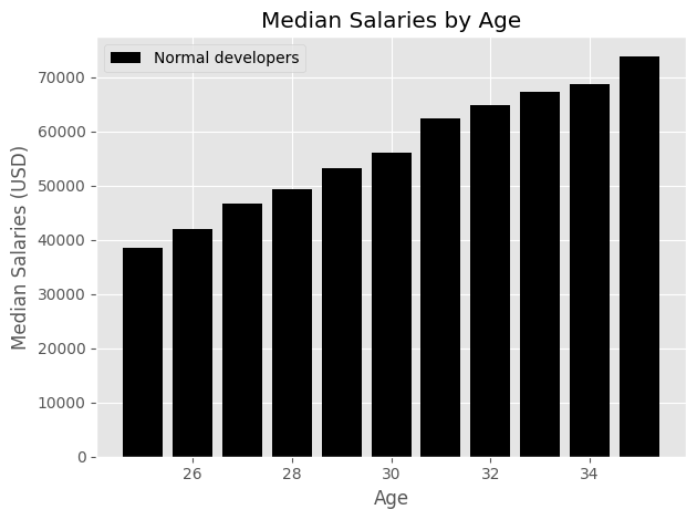
ages_x = [25,26,27,28,29,30,31,32,33,34,35]
dev_y = [38496, 42000, 46752, 49320, 53200, 56000, 62316, 64928, 67317, 68748, 73752]
py_dev_y = [45372, 48476, 53850, 57287, 63016, 65998, 70003, 70000, 71496, 75370, 83640]
js_dev_y = [37810, 43515, 46823, 49293, 53437, 56373, 62375, 66674, 68745, 68746, 74583]
plt.style.use("ggplot")
plt.plot(ages_x, py_dev_y, color = "#5a7d9a", linestyle = '-',linewidth = 4, label = "Python_Developers")
plt.plot(ages_x, js_dev_y, color = "#adad3b", linestyle = '-',linewidth = 4, label = "Java_script_Developers")
plt.bar(ages_x, dev_y, color = "k", linestyle = "--", label = "Normal developers")
plt.title("Median Salaries by Age")
plt.xlabel("Age")
plt.ylabel("Median Salaries (USD)")
plt.legend()
plt.tight_layout()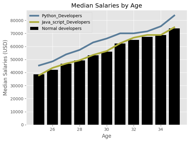
Side-by-side
ages_x = [25,26,27,28,29,30,31,32,33,34,35]
dev_y = [38496, 42000, 46752, 49320, 53200, 56000, 62316, 64928, 67317, 68748, 73752]
py_dev_y = [45372, 48476, 53850, 57287, 63016, 65998, 70003, 70000, 71496, 75370, 83640]
js_dev_y = [37810, 43515, 46823, 49293, 53437, 56373, 62375, 66674, 68745, 68746, 74583]
plt.style.use("ggplot")
plt.bar(ages_x, py_dev_y, color = "#5a7d9a", linestyle = '-',linewidth = 4, label = "Python_Developers")
plt.bar(ages_x, js_dev_y, color = "#adad3b", linestyle = '-',linewidth = 4, label = "Java_script_Developers")
plt.bar(ages_x, dev_y, color = "k", linestyle = "--", label = "Normal developers")
plt.title("Median Salaries by Age")
plt.xlabel("Age")
plt.ylabel("Median Salaries (USD)")
plt.legend()
plt.tight_layout()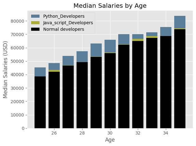
ages_x = [25,26,27,28,29,30,31,32,33,34,35]
x_index = np.arange(len(ages_x))
width = 0.25
dev_y = [38496, 42000, 46752, 49320, 53200, 56000, 62316, 64928, 67317, 68748, 73752]
py_dev_y = [45372, 48476, 53850, 57287, 63016, 65998, 70003, 70000, 71496, 75370, 83640]
js_dev_y = [37810, 43515, 46823, 49293, 53437, 56373, 62375, 66674, 68745, 68746, 74583]
plt.style.use("ggplot")
plt.bar(x_index - width, py_dev_y, width = width, color = "#5a7d9a", linestyle = '-', label = "Python_Developers")
plt.bar(x_index, js_dev_y, width = width, color = "#adad3b", linestyle = '-', label = "Java_script_Developers")
plt.bar(x_index + width, dev_y, width = width, color = "k", linestyle = "--", label = "Normal developers")
plt.title("Median Salaries by Age")
plt.xlabel("Age")
plt.ylabel("Median Salaries (USD)")
plt.legend()
plt.tight_layout()
# plt.xticks()
ages_x = [25,26,27,28,29,30,31,32,33,34,35]
x_index = np.arange(len(ages_x)) # creating an index value np array for each value of age
width = 0.25
dev_y = [38496, 42000, 46752, 49320, 53200, 56000, 62316, 64928, 67317, 68748, 73752]
py_dev_y = [45372, 48476, 53850, 57287, 63016, 65998, 70003, 70000, 71496, 75370, 83640]
js_dev_y = [37810, 43515, 46823, 49293, 53437, 56373, 62375, 66674, 68745, 68746, 74583]
plt.style.use("ggplot")
plt.bar(x_index - width, py_dev_y, width = width, color = "#5a7d9a", linestyle = '-', label = "Python_Developers")
plt.bar(x_index, js_dev_y, width = width, color = "#adad3b", linestyle = '-', label = "Java_script_Developers")
plt.bar(x_index + width, dev_y, width = width, color = "k", linestyle = "--", label = "Normal developers")
plt.title("Median Salaries by Age")
plt.xticks(ticks = x_index, labels = ages_x)
plt.xlabel("Age")
plt.ylabel("Median Salaries (USD)")
plt.legend()
plt.tight_layout()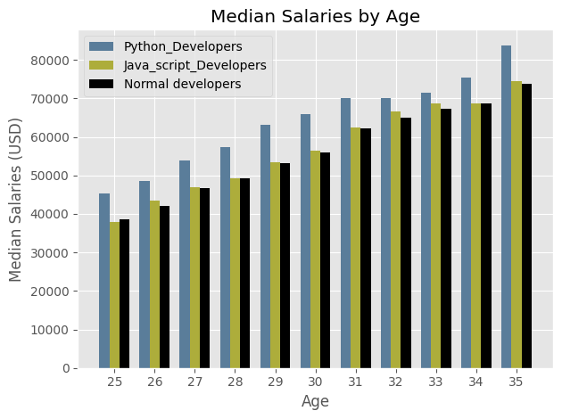
barh
data = pd.read_csv("data/data.csv")
data.head()| Responder_id | LanguagesWorkedWith | |
|---|---|---|
| 0 | 1 | HTML/CSS;Java;JavaScript;Python |
| 1 | 2 | C++;HTML/CSS;Python |
| 2 | 3 | HTML/CSS |
| 3 | 4 | C;C++;C#;Python;SQL |
| 4 | 5 | C++;HTML/CSS;Java;JavaScript;Python;SQL;VBA |
ids = data["Responder_id"]
lang_responses = data["LanguagesWorkedWith"]
from collections import Counter
lang_counter = Counter()
for response in lang_responses:
lang_counter.update(response.split(";"))lang_counterCounter({'JavaScript': 59219,
'HTML/CSS': 55466,
'SQL': 47544,
'Python': 36443,
'Java': 35917,
'Bash/Shell/PowerShell': 31991,
'C#': 27097,
'PHP': 23030,
'C++': 20524,
'TypeScript': 18523,
'C': 18017,
'Other(s):': 7920,
'Ruby': 7331,
'Go': 7201,
'Assembly': 5833,
'Swift': 5744,
'Kotlin': 5620,
'R': 5048,
'VBA': 4781,
'Objective-C': 4191,
'Scala': 3309,
'Rust': 2794,
'Dart': 1683,
'Elixir': 1260,
'Clojure': 1254,
'WebAssembly': 1015,
'F#': 973,
'Erlang': 777})language = []
popularity = []
for item in lang_counter.most_common(15):
language.append(item[0])
popularity.append(item[1])print(language)
print(popularity)['JavaScript', 'HTML/CSS', 'SQL', 'Python', 'Java', 'Bash/Shell/PowerShell', 'C#', 'PHP', 'C++', 'TypeScript', 'C', 'Other(s):', 'Ruby', 'Go', 'Assembly']
[59219, 55466, 47544, 36443, 35917, 31991, 27097, 23030, 20524, 18523, 18017, 7920, 7331, 7201, 5833]plt.bar(language, popularity)
plt.title("Popularity of Programming languages")
plt.ylabel("Popularity")
plt.xlabel("Programming language")Text(0.5, 0, 'Programming language')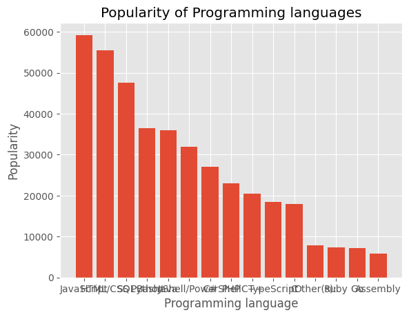
# 위의 그래프에서 X축 label이 명확하지 않다는 것을 알 수 있습니다. 따라서 가로 막대 그래프를 사용합니다.
plt.barh(language, popularity)
plt.title("Popularity of Programming languages")
plt.xlabel("Popularity")
plt.ylabel("Programming language")
Text(0, 0.5, 'Programming language')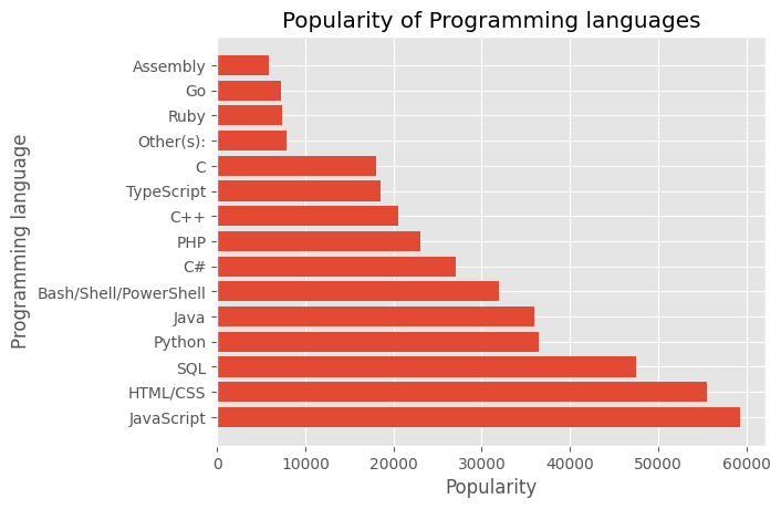
# 가장 인기 있는 언어를 상단에 유지하여 막대 그래프를 반전시킬 수 있습니다.
language.reverse()
popularity.reverse()
plt.barh(language, popularity)
plt.title("Popularity of Programming languages")
plt.xlabel("Popularity")
plt.ylabel("Programming language")
Text(0, 0.5, 'Programming language')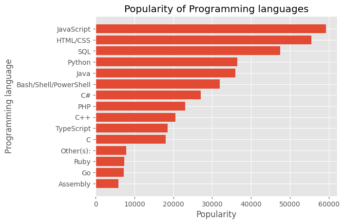
Scatter Plots
import pandas as pd
import matplotlib.pyplot as plt
x = [5,7,8,5,6,7,9,2,3,4,4,4,2,6,3,6,8,6,4,1]
y = [7,4,3,9,1,3,2,5,2,4,8,7,1,6,4,9,7,7,5,1]
plt.scatter(x,y)
plt.tight_layout()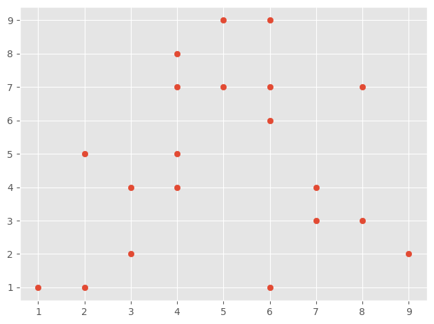
Customizing the scatter plots
# 점의 크기 변경
x = [5,7,8,5,6,7,9,2,3,4,4,4,2,6,3,6,8,6,4,1]
y = [7,4,3,9,1,3,2,5,2,4,8,7,1,6,4,9,7,7,5,1]
plt.scatter(x,y, s = 200)
plt.tight_layout()
# 점의 색상 변경
x = [5, 7, 8, 5, 6, 7, 9, 2, 3, 4, 4, 4, 2, 6, 3, 6, 8, 6, 4, 1]
y = [7, 4, 3, 9, 1, 3, 2, 5, 2, 4, 8, 7, 1, 6, 4, 9, 7, 7, 5, 1]
plt.scatter(x, y, s=150, color="green")
plt.tight_layout()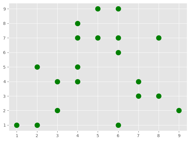
# 그래프의 마커 변경하기
x = [5,7,8,5,6,7,9,2,3,4,4,4,2,6,3,6,8,6,4,1]
y = [7,4,3,9,1,3,2,5,2,4,8,7,1,6,4,9,7,7,5,1]
plt.scatter(x,y, s = 150, color = "green", marker = "X")
plt.tight_layout()
# 마커에 가장자리와 알파값 부여하기
x = [5,7,8,5,6,7,9,2,3,4,4,4,2,6,3,6,8,6,4,1]
y = [7,4,3,9,1,3,2,5,2,4,8,7,1,6,4,9,7,7,5,1]
plt.scatter(x,y, s = 150, c = "green", edgecolor = "black", linewidth = 2, alpha = 0.75)
plt.tight_layout()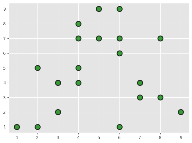
Using differnt colors for markers.
x = [5,7,8,5,6,7,9,2,3,4,4,4,2,6,3,6,8,6,4,1]
y = [7,4,3,9,1,3,2,5,2,4,8,7,1,6,4,9,7,7,5,1]
colors = [7,5,3,9,5,7,2,5,3,7,1,2,8,1,9,2,5,6,7,5]
plt.scatter(x,y, s = 150, c = colors, cmap = "Reds", edgecolor = "black", linewidth = 2, alpha = 0.75)
plt.tight_layout()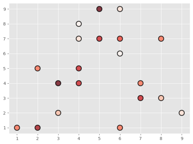
# Setting a colorbar legend
x = [5, 7, 8, 5, 6, 7, 9, 2, 3, 4, 4, 4, 2, 6, 3, 6, 8, 6, 4, 1]
y = [7, 4, 3, 9, 1, 3, 2, 5, 2, 4, 8, 7, 1, 6, 4, 9, 7, 7, 5, 1]
colors = [7, 5, 3, 9, 5, 7, 2, 5, 3, 7, 1, 2, 8, 1, 9, 2, 5, 6, 7, 5]
plt.scatter(
    x, y, s=150, c=colors, cmap="Reds", edgecolor="black", linewidth=2, alpha=0.75
)
cbar = plt.colorbar()
cbar.set_label("Satisfaction Ratings")
plt.tight_layout()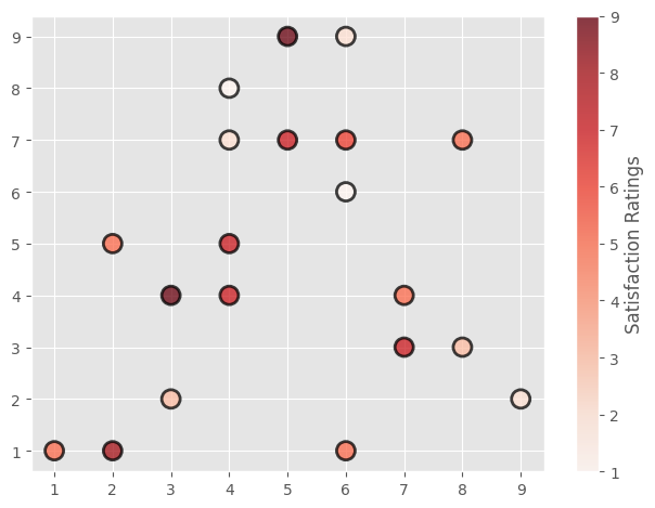
x = [5,7,8,5,6,7,9,2,3,4,4,4,2,6,3,6,8,6,4,1]
y = [7,4,3,9,1,3,2,5,2,4,8,7,1,6,4,9,7,7,5,1]
colors = [7,5,3,9,5,7,2,5,3,7,1,2,8,1,9,2,5,6,7,5]
sizes = [209,486,381,255,717,315,175,228,174,592,293,399,255,525,154,253,475,457,214,253]
plt.scatter(x,y, s = sizes, c = colors, cmap = "Reds", edgecolor = "black", linewidth = 2, alpha = 0.75)
cbar = plt.colorbar()
cbar.set_label("Satisfaction Ratings")
plt.tight_layout()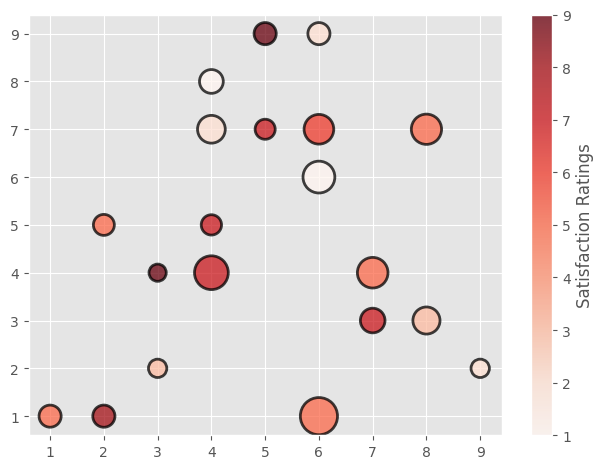
Scatter plot for a CSV file data
import pandas as pd
import matplotlib.pyplot as plt
data = pd.read_csv("data/yt.csv")
data.head()| view_count | likes | ratio | |
|---|---|---|---|
| 0 | 8036001 | 324742 | 96.91 |
| 1 | 9378067 | 562589 | 98.19 |
| 2 | 2182066 | 273650 | 99.38 |
| 3 | 6525864 | 94698 | 96.25 |
| 4 | 9481284 | 582481 | 97.22 |
# 조회 수에 따라 좋아요 수가 증가하는지 확인

views = data["view_count"]
likes = data["likes"]
ratio = data["ratio"]

plt.scatter(views, likes, edgecolor = "black", linewidth = 2, alpha = 0.75)

plt.title("Trending Youtube videos")
plt.xlabel("Number of views")
plt.ylabel("Number of likes")

plt.tight_layout()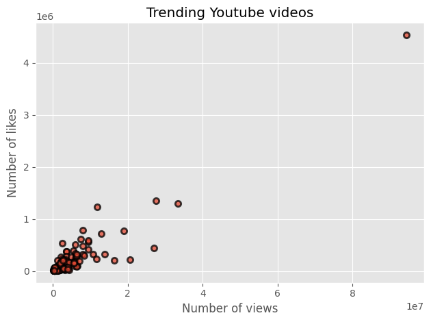
views = data["view_count"]
likes = data["likes"]
ratio = data["ratio"]

plt.scatter(views, likes, edgecolor = "black", linewidth = 2, alpha = 0.75)

plt.title("Trending Youtube videos")
plt.xlabel("Number of views")
plt.ylabel("Number of likes")

plt.xscale("log")
plt.yscale("log")
plt.tight_layout()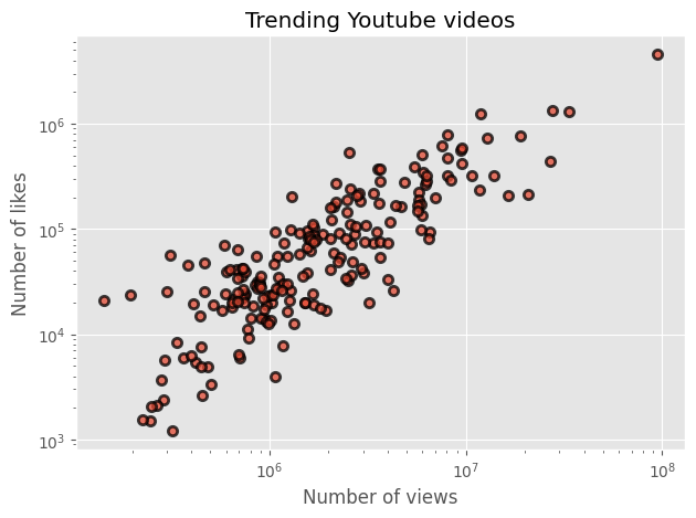
# 좋아요/싫어요 비율을 색상 매개변수로 사용하여 데이터를 더 잘 설명할 수 있음

views = data["view_count"]
likes = data["likes"]
ratio = data["ratio"]

plt.scatter(views, likes, c = ratio, cmap = "summer", edgecolor = "black", linewidth = 2, alpha = 0.75)

cbar = plt.colorbar()
cbar.set_label("Like to Dislike Ratio")

plt.title("Trending Youtube videos")
plt.xlabel("Number of views")
plt.ylabel("Number of likes")

plt.xscale("log")
plt.yscale("log")
plt.tight_layout()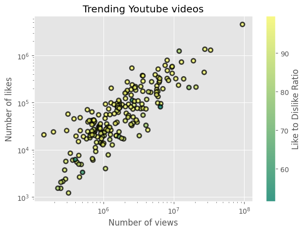
Plotting Time Series Data
import pandas as pd
import matplotlib.pyplot as plt
import matplotlib.dates as mpl_dates
from datetime import datetime, timedelta
date = [
datetime (2019,5,24),
datetime (2019,5,25),
datetime (2019,5,26),
datetime (2019,5,27),
datetime (2019,5,28),
datetime (2019,5,29),
datetime (2019,5,30)
]
y = [0,1,3,4,6,5,7]
plt.plot(date, y)
date = [
    datetime (2019,5,24),
    datetime (2019,5,25),
    datetime (2019,5,26),
    datetime (2019,5,27),
    datetime (2019,5,28),
    datetime (2019,5,29),
    datetime (2019,5,30)
]

y = [0,1,3,4,6,5,7]

plt.plot(date, y, linestyle = "solid")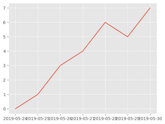
date = [
    datetime (2019,5,24),
    datetime (2019,5,25),
    datetime (2019,5,26),
    datetime (2019,5,27),
    datetime (2019,5,28),
    datetime (2019,5,29),
    datetime (2019,5,30)
]

y = [0,1,3,4,6,5,7]

plt.plot(date, y, linestyle = "solid")
plt.gcf().autofmt_xdate() # gcf (get current figure) autofmt(auto format)
plt.tight_layout()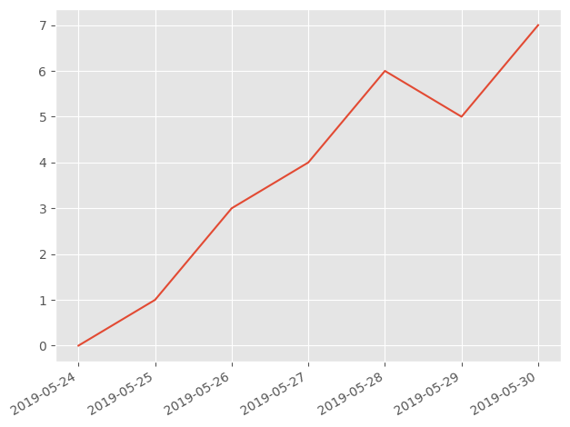
Changing the format of dates
date = [
    datetime (2019,5,24),
    datetime (2019,5,25),
    datetime (2019,5,26),
    datetime (2019,5,27),
    datetime (2019,5,28),
    datetime (2019,5,29),
    datetime (2019,5,30)
]

y = [0,1,3,4,6,5,7]

plt.plot(date, y, linestyle = "solid")
plt.gcf().autofmt_xdate()
date_format = mpl_dates.DateFormatter("%d, %b,%Y")
plt.gca().xaxis.set_major_formatter(date_format) # gca = get current axis
plt.tight_layout()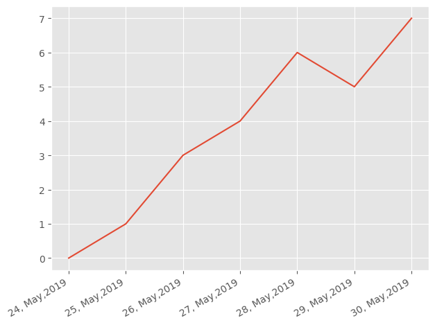
Using the datetime Plot on CSV file
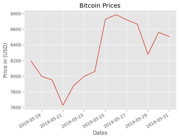
data = pd.read_csv("data/datetime.csv")data.head()| Date | Open | High | Low | Close | Adj Close | Volume | |
|---|---|---|---|---|---|---|---|
| 0 | 2019-05-18 | 7266.080078 | 8281.660156 | 7257.259766 | 8193.139648 | 8193.139648 | 723011166 |
| 1 | 2019-05-19 | 8193.139648 | 8193.139648 | 7591.850098 | 7998.290039 | 7998.290039 | 637617163 |
| 2 | 2019-05-20 | 7998.290039 | 8102.319824 | 7807.770020 | 7947.930176 | 7947.930176 | 357803946 |
| 3 | 2019-05-21 | 7947.930176 | 8033.759766 | 7533.660156 | 7626.890137 | 7626.890137 | 424501866 |
| 4 | 2019-05-22 | 7626.890137 | 7971.259766 | 7478.740234 | 7876.500000 | 7876.500000 | 386766321 |
price_date = data["Date"]
price_close = data["Close"]
plt.plot(price_date, price_close, linestyle = "solid")
plt.gcf().autofmt_xdate()
plt.title("Bitcoin Prices")
plt.xlabel("Dates")
plt.ylabel("Price in (USD)")Text(0, 0.5, 'Price in (USD)')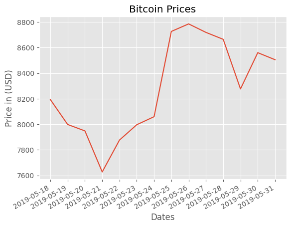
# We are making use of pandas to_datetime method
data["Date"] = pd.to_datetime(data["Date"])
data.sort_values('Date', inplace = True)
price_date = data["Date"]
price_close = data["Close"]
plt.plot(price_date, price_close, linestyle = "solid")
plt.gcf().autofmt_xdate()
plt.title("Bitcoin Prices")
plt.xlabel("Dates")
plt.ylabel("Price in (USD)")
Text(0, 0.5, 'Price in (USD)')